In this post we are going to through fitting a line of best fit using python. If you just want the python code feel free to just read the first section.
Note: This post assumes you didn’t do much maths at university/college, or that you just forgot! It serves as a starter for future, more challenging posts!
This first post has two basic aims:
- Give some simple code to make some lines
- Spark an interest and understanding of why aim 1 in isolation isn’t a particularly good idea
Give me a straight line already:
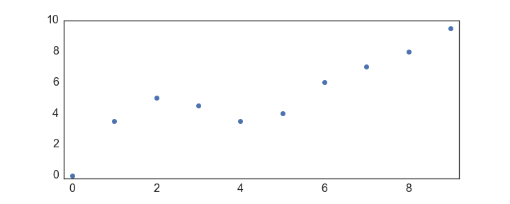
Let’s first import our modules and make some data.
import numpy as np
import matplotlib.pyplot as plt

y = np.array([0,3.5,5,4.5,3.5,4,6,7,8,9.5])
x = np.arange(y.shape[0])

plt.plot(x,y, 'o')
Then, probably the easiest way to get yourself a line is with numpy’s polyfit function:
def give_me_a_straight_line(x,y):
    w, b  = np.polyfit(x,y,deg=1)
    line  = w * x + b
    return line

line = give_me_a_straight_line(x,y)

plt.plot(x,y,'o')
plt.plot(x,line,'r--')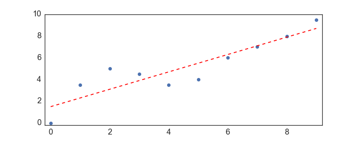
There: if all you wanted was the code for a straight line through your data, you should be all set! …However, we should really talk about what you are actually doing with this code. You are approximating a function of the following form:
\[\mathbf{y} \approx w\mathbf{x} + b\]Where:
$\mathbf{x}$ is a $N$ dimensional vector of x values (think list or 1D-array)
$\mathbf{y}$ is a $N$ dimensional vector of y values
$w$ is a scalar that weights the $x$ value
$b$ is a scalar offset or bias (intercept)
In essence, the two parameters you are fitting, $w$ & $b$, are combined with an $x$ value to predict what a corresponding $y$ value should be. How does np.polyfit do this? Well, the fitting procedure that np.polyfit uses is least squares, which has a neat solution:
\[(\mathbf{X}^T\mathbf{X})^{-1}\mathbf{X}^{T}\mathbf{y} = \mathbf{\beta}\]Wait, what? Don’t worry, we’ll go through how we get to this “neat solution” in the next post, but for now, why has $\mathbf{x}$ changed to $\mathbf{X}$ and what is $\mathbf{\beta}$?
First, $\mathbf{\beta}$ : this is now a vector (similar to a list), and it looks like $[w, b]^T$ - it’s a column vector, hence the $^T$. Therefore $\mathbf{\beta}$[0] will give you your x-weight, $w$, and $\mathbf{\beta}$[1] your bias, $b$.
Second, $\mathbf{X}$ is a matrix (similar to an array), with two columns: the orginal $\mathbf{x}$ vector, which has now also been augmented by an equally long column of ones that are used to fit the $b$ parameter.
Let’s plug this into our function already!
def give_me_a_straight_line_without_polyfit(x,y):

    # first augment the x vector with ones
    ones_vec = np.ones(x.shape)
    X = np.vstack([x, ones_vec]).T #.T as we want two columns

    # now plugin our least squares "solution"
    XX   = np.linalg.inv(np.dot(X.T, X))
    Xt_y = np.dot(X.T, y.T) #y.T as we want column vector
    beta = np.dot(XX, Xt_y)

    line = beta[0]*x + beta[1]
    return line

line = give_me_a_straight_line_without_polyfit(x,y)
plt.plot(x,y, 'o')
plt.plot(x,line, 'r--')

Okay, so that’s all good, but what if you want a curvey line of best fit, to join up the points…?
Give me a line that goes nicely through my points:
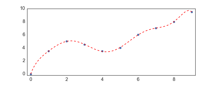
If you want that we can just dial up and down the polynomial degree argument in polyfit…:
Note small edits to the code here! We now return a convenience object from the function, which allows us to pass in new xvalues
def give_me_a_line_like_excel(x,y):
    coefs = np.polyfit(x,y,deg=8)
    p_obj = np.poly1d(coefs) #this is a convenience class
    return p_obj

p_obj = give_me_a_line_like_excel(x,y)
x_line = np.linspace(min(x), max(x), 100) #make new xvalues
y_line = p_obj(x_line)

plt.plot(x,y,'o')
plt.plot(x_line,y_line, 'r--')

So what’s going on here?
We are now still predicting what the corresponding $y$ should be for a given $x$, but instead of doing this with the simple:
\[y = wx + b\]We are now augmenting our $x$’s by raising them to powers from 0 - to our polynomial degree, and using seperate fitted coefcients for each of these $x$’s.
\[y = w_0x^0 + w_1x^1 + w_2x^2 + ... + w_{p-1}x^{p-1}+ w_{p}x^{p}\]This can be better expressed using a summation sign:
\[y = \sum_{i = 0}^{p} w_ix^i\]Note, that we will not have to explicitly add a $b$ for our interecept, this is inbuilt in the expression as $x^0 = 1$, and therefore $w_0 = b$.
What we have actually done is to construct what is a called a Vandermonde matrix $\mathbf{X}^{N\times P}$ from a $N$ dimensional vector, $\mathbf{x}$. In a Vandermonde matrix, each column is the orginal $\mathbf{x}$, raised element-wise to a power, up to the $p^{th}$ degree of the polynomial that we want to fit.
\[\mathbf{V} = \begin{bmatrix} x_1^0 & x_1 & x_1^2 & x_1^3 &\cdots & x_1^p \\ x_2^0 & x_2 & x_2^2 & x_2^3 &\cdots & x_2^p \\ \vdots&\vdots&\vdots&\vdots& \ddots & \vdots \\ x_N^0 & x_N & x_N^2 & x_N^3 &\cdots & x_N^p \end{bmatrix}\]Therefore, in matrix notation (like the least squares solution above), the equation that we are using to find a predicted $y$ from an $x$ value is:
\[\mathbf{y} = \mathbf{X}\mathbf{\beta}\]Where:
$\mathbf{y}$ is the original vector of target $y$ values
$\mathbf{X}$ is a Vandermonde matrix constructed from the original $\mathbf{x}$
$\mathbf{\beta}$ is our vector of weights, or coefficients
Don’t worry if you’ve not done/forgotten what happens when a vector and matrix meet. Above is just a concise way of writing $ \sum_{i}^{n}y_i = \sum_{i}^{n}w_0x_i^0 + w_1x_i^1 + … + + w_{p}x_i^{p}$. So we are just looping through all of the datapoints in the $\mathbf{y}$ and original $\mathbf{x}$ vectors.
Okay, well know we know this, we don’t need np.polyfit!
- note the pretty cool use of a closure, to replicate the np.poly1d() call functionality
def give_me_a_line_like_excel_without_polyfit(x,y, deg = 8):

    deg += 1 # just to replicate np.polyfits deg argument

    # construct a matrix of polynomials
    X = np.vander(x, deg)

    # now plugin our least squares "solution"
    XX   = np.linalg.inv(np.dot(X.T, X))
    Xt_y = np.dot(X.T, y.T)
    beta = np.dot(XX, Xt_y)

    # make a python closure to replicate the behaviour of np.poly1d
    def my_p_obj(new_x):
        # first we make our X matrix
        X = np.vander(new_x, deg)

        # now loop through our coffecients to get new_y vector
        line_best_fit = np.zeros(new_x.shape)
        for col_i,weight in enumerate(beta[:-1]):
            line_best_fit += weight*X[:,col_i]
        line_best_fit += beta[-1]

        return line_best_fit

    # return our closure function
    return my_p_obj


my_p_obj = give_me_a_line_like_excel_without_polyfit(x,y)

x_line = np.linspace(min(x), max(x), 100)
y_line = my_p_obj(x_line)

plt.plot(x,y, 'o')
plt.plot(x_line,y_line, 'r--')
p.s. It’s probably worth noting that in practice, people don’t actually invert $X^TX$ so directly. Instead, you should use things like np.linalg.lstsq().